Copula: A Very Short Introduction
You might have seen the following true/false questions in the final exam of your first statistics course.
- If \( (Z_1, Z_2) \) follows a bivariate Gaussian distribution, do \( Z_1 \) and \( Z_2 \) follow univariate Gaussian distributions?
- If \( Z_1 \) and \( Z_2 \) follow univariate Gaussian distributions, does \( (Z_1, Z_2) \) follow a bivariate Gaussian distribution?
The answer to the first question is true and to the second is false. “What could the joint distribution of \( (Z_1, Z_2) \) be, if \( Z_1 \) and \( Z_2 \) are univariate Gaussians?”, you may ask.
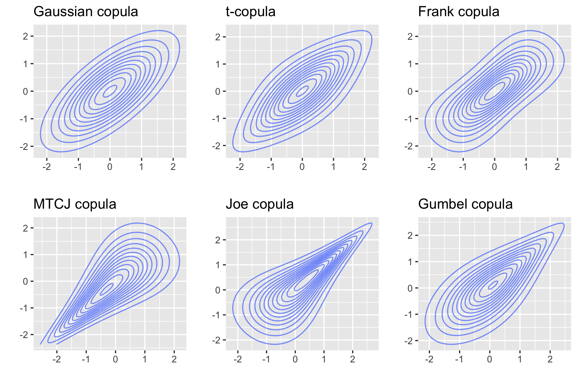
Figure 1 shows the contour plots for different bivariate distributions where \(Z_1\) and \(Z_2\) follow standard Gaussian distributions. All of them are constructed using copulas, which are a flexible tool to model the dependence among random variables. In this post, I give a short introduction to (bivariate) copulas. Other references on this topic include an introduction by Schmidt (2007) and a monograph by my Ph.D. advisor Joe (2014).
1. Copula–a first glance
Consider a continuous random vector \((X_1, X_2)\). Let \(F_j\) be the marginal cumulative distribution function (CDF) of \(X_j\) for \(j=1,2\), and \(F\) be the joint CDF. We apply the probability integral transform and define \(U_j := F_j(X_j)\). Since \(X_j\) is assumed to be continuous, \(U_j \sim \mathcal{U}(0,1) \) follows a uniform distribution. Then the CDF of \((U_1, U_2)\) is the copula of \((X_1, X_2)\), denoted by \(C\). $$C(u_1, u_2) = \mathbb{P}(U_1 \leq u_1, U_2 \leq u_2).$$ The joint distribution can be then decomposed into two components: the copula and marginals: \begin{align} F(x_1, x_2) &= \mathbb{P}(X_1 \leq x_1, X_2 \leq x_2) \newline &= \mathbb{P}(U_1 \leq F_1(x_1), U_2 \leq F_2(x_2)) \newline &= C(F_1(x_1), F_2(x_2)). \end{align}
The name “copula” comes from the Latin for “link”; it links the marginals to the joint distribution.
We first consider a few simple copulas.
Example 1 (Independence copula). Let \(X_1\) and \(X_2\) be independent random variables. The corresponding copula is \begin{align} C(u_1, u_2) &= \mathbb{P}(U_1 \leq u_1, U_2 \leq u_2) \newline &= \mathbb{P}(U_1 \leq u_1) \mathbb{P}(U_2 \leq u_2) \newline &= u_1 u_2. \end{align} The second equality is due to independence of \(U_1\) and \(U_2\), and the last equality is because \(U_1\) and \(U_2\) follow uniform distributions.
Example 2 (Comonotonicity copula). Let \(X_2 = 2X_1\); that is, \(X_1\) and \(X_2\) have a deterministic and positive relationship. We can derive the relation between the CDFs: $$F_1(x) = \mathbb{P}(X_1 \leq x) = \mathbb{P}(2 X_1 \leq 2 x) = \mathbb{P}(X_2 \leq 2x) = F_2(2x),$$ which leads to the fact that \(U_1\) is equal to \(U_2\): $$U_1 = F_1(X_1) = F_2(2 X_1) = F_2(X_2) = U_2.$$ The copula is \begin{align} C(u_1, u_2) &= \mathbb{P}(U_1 \leq u_1, U_2 \leq u_2) \newline &= \mathbb{P}(U_1 \leq u_1, U_1 \leq u_2) \newline &= \mathbb{P}(U_1 \leq \min \{u_1, u_2\}) \newline &= \min \{u_1, u_2\}. \end{align} The comonotonicity copula has perfect positive dependence. Note that \(X_2 = 2X_1\) can be replaced by \(X_2 = T(X_1)\) for any strictly increasing transformation \(T\).
Example 3 (Countermonotonicity copula). Similar to the previous example, we consider the perfect negative dependence. Let \(X_2 = -2X_1\), then $$F_1(x) = \mathbb{P}(X_1 \leq x) = \mathbb{P}(-2 X_1 \geq -2x) = \mathbb{P}(X_2 \geq -2x) = 1 - F_2(-2x),$$ and $$U_1 = F_1(X_1) = 1-F_2(-2X_1) = 1-F_2(X_2) = 1-U_2.$$ The copula is \begin{align} C(u_1, u_2) &= \mathbb{P}(U_1 \leq u_1, U_2 \leq u_2) \newline &= \mathbb{P}(U_1 \leq u_1, 1-U_1 \leq u_2) \newline &= \mathbb{P}(1 - u_2 \leq U_1 \leq u_1) \newline &= \max \{u_1 + u_2 - 1, 0\}. \end{align} The countermonotonicity copula is the copula of \(X_2 = T(X_1)\) for any strictly decreasing transformation \(T\).
Example 4 (Bivariate Gaussian copula). The previous examples are all extreme cases, with either perfect dependence or independence. We now introduce a copula that is derived from the bivariate Gaussian distribution. Consider $$\begin{pmatrix} X_1 \newline X_2 \end{pmatrix} \sim \mathcal{N} \left( \begin{pmatrix} 0 \newline 0 \end{pmatrix} , \begin{pmatrix} 1 & \rho \newline \rho & 1 \end{pmatrix} \right).$$ The copula is \begin{align} C(u_1, u_2) &= \mathbb{P}(U_1 \leq u_1, U_2 \leq u_2) \newline &= \mathbb{P}(X_1 \leq \Phi^{-1}(u_1), X_2 \leq \Phi^{-1}(u_2)) \newline &= \Phi_2(\Phi^{-1}(u_1), \Phi^{-1}(u_2); \rho), \end{align} where \(\Phi\) is the CDF of a standard normal distribution and \(\Phi_2(\cdot; \rho)\) is the joint CDF of \((X_1, X_2)\). Also different from the previous example, this is the first parametric copula family we have introduced. The Gaussian copula has a parameter \(\rho\) controlling the strength of dependence.
2. Common parametric copula families
We now give a more general definition of bivariate copulas.
Definition 1. A bivariate copula \(C: [0,1]^2 \to [0,1]\) is a function which is a bivariate cumulative distribution function with uniform marginals.
The copulas we have introduced so far are all derived from bivariate distributions. In other words, it goes from the joint distribution \(F\) on the left-hand side of the following equation to the copula \(C\) and marginals \(F_j\) on the right-hand side. $$F(x_1, x_2) = C(F_1(x_1), F_2(x_2)).$$
Given the general definition of the copula, some copula families \(C\) can further be defined explicitly. This allows us to go from the right-hand side to the left-hand side; that is, linking two marginals using a copula to get a joint distribution.
Below are shown some commonly used parametric bivariate copula families, where \(\rho, \nu\) and \(\delta\) are the parameters.
| Copula family | Copula CDF |
|---|---|
| Gaussian | \(\Phi_2 \left( \Phi^{-1}(u_1), \Phi^{-1}(u_2); \rho \right)\) |
| t | \( T_{2, \nu} \left(T_{1, \nu}^{-1}(u_1), T_{1, \nu}^{-1}(u_2); \rho \right) \) |
| Frank | \( -\delta^{-1} \log \left( \frac{1 - e^{-\delta} - (1 - e^{-\delta u_1}) (1 - e^{-\delta u_2})} {1-e^{-\delta}} \right) \) |
| MTCJ | \( (u_1^{-\delta} + u_2^{-\delta} - 1)^{-1/\delta} \) |
| Joe | \( 1 - \left( (1-u_1)^{\delta} + (1-u_2)^{\delta} - (1-u_1)^{\delta} (1-u_2)^{\delta} \right)^{1/\delta} \) |
| Gumbel | \( \exp \left( -\left( (-\log u_1)^{\delta} + (-\log u_2)^{\delta} \right)^{1/\delta} \right) \) |
Figure 1 shows the constructed bivariate joint distributions using the copula families above and univariate standard normal distributions (i.e., \(F_1 = F_2 = \Phi\)).
3. Fréchet–Hoeffding bounds
As hinted before, the comonotonicity and countermonotonicity copulas are two extreme cases: perfect positive dependence and perfect negative dependence. This is formally stated by the following theorem.
Theorem 1 (Fréchet–Hoeffding bounds).
For any copula \( C:[0,1]^2 \to [0,1] \) and any \( (u_1, u_2) \in [0,1]^2 \), the following bounds hold: $$\max \{ u_1+u_2-1, 0 \} \leq C(u_1, u_2) \leq \min \{ u_1, u_2 \}.$$
Figure 2 shows the upper and lower bounds in green and blue respectively. By the theorem, every copula lies between the two surfaces.
4. Reflected copula
Given \( (U_1, U_2) \sim C \), the reflected copula \(\widehat{C}\) is defined as the copula of \( (1-U_1, 1-U_2) \). That is, \begin{align} \widehat{C}(u_1, u_2) &= \mathbb{P}(1 - U_1 \leq u_1, 1 - U_2 \leq u_2) \newline &= \mathbb{P}(U_1 \geq 1 - u_1, U_2 \geq 1 - u_2). \end{align}
The reflected copula \(\widehat{C}\) is handy when studying the upper and lower tail properties of a copula, as we will see later. To facilitate the analysis, we calculate the following probability (survival function): \begin{align} \mathbb{P}(U_1 > v_1, U_2 > v_2) &= 1 - \mathbb{P}(U_1 \leq v_1 \mbox{ or } U_2 \leq v_2) \newline &= 1 - \mathbb{P}(U_1 \leq v_1) - \mathbb{P}(U_2 \leq v_2) + \mathbb{P}(U_1 \leq v_1, U_2 \leq v_2) \newline &= 1 - v_1 - v_2 + C(v_1, v_2). \end{align} The second equality is due to the inclusion–exclusion principle. Finally, we have $$\widehat{C}(u_1, u_2) = u_1 + u_2 - 1 + C(1-u_1, 1-u_2).$$
5. Rank correlations
Correlation coefficients are useful in summarizing the dependence structure between two variables using a single number. Pearson’s correlation is probably the most commonly used one. However, it is known that Pearson’s correlation between \(X\) and \(X^2\) is zero for \(X \sim \mathcal{N} (0, 1)\). This is often used as an example to illustrate that Pearson’s correlation only measures linear correlation; it is not invariant under increasing transformations.
In nonparametric statistics, rank correlations, such as Spearman’s rho and Kendall’s tau, are defined by the ranks of the data rather than the data itself. As a result, they are invariant under increasing transformations. Since copulas are also independent of marginals, there should be a natural connection between copulas and rank correlations. In fact, both Spearman’s rho and Kendall’s tau can be defined directly as functionals of a copula.
-
Spearman’s rho: $$ \rho_S( C ) = \iint_{[0,1]^2} uv \, \mathrm{d} C(u, v) -3. $$
-
Kendall’s tau: $$ \rho_\tau( C ) = \iint_{[0,1]^2} C(u, v) \, \mathrm{d} C(u, v). $$
The integrals are Riemann–Stieltjes integrals.
The parameters of bivariate copulas in Figure 1 are chosen such that their Kendall’s tau all equals 0.5.
6. Tail dependence
Apart from correlation coefficients, the coefficient of tail dependence is also an essential measure of dependence. It characterizes the dependence of a bivariate distribution in the extremes, which is important in many financial applications.
Consider the following bivariate Gaussian distribution $$\begin{pmatrix} X_1 \newline X_2 \end{pmatrix} \sim \mathcal{N} \left( \begin{pmatrix} 0 \newline 0 \end{pmatrix} , \begin{pmatrix} 1 & 0.5 \newline 0.5 & 1 \end{pmatrix} \right).$$ We are interested in the conditional probability \(\mathbb{P}(X_2>t | X_1>t)\); that is, given the event that \(X_1\) is greater than a threshold \(t\), what is the probability that \(X_2\) is also greater than \(t\).
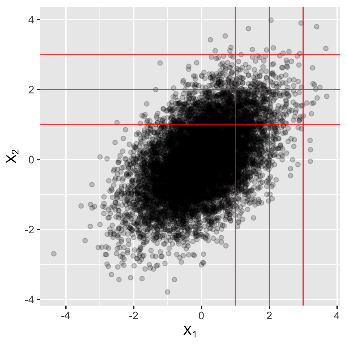
Figure 3 shows 10,000 random samples from the distribution. For \(t \in \{1,2,3\}\), the probability can be visually estimated: among the points to the right of \(x=t\), how many of them are above \(y=t\). It appears that the probability decreases as \(t\) increases. A further numerical calculation gives
- \(\mathbb{P}(X_2>1 | X_1>1) = 0.39, \)
- \(\mathbb{P}(X_2>2 | X_1>2) = 0.18, \)
- \(\mathbb{P}(X_2>3 | X_1>3) = 0.06. \)
It can be shown that $$\lim_{t \to +\infty}\mathbb{P}(X_2>t | X_1>t) = 0. $$
Interestingly, although \(X_1\) and \(X_2\) are correlated, they behave like independent random variables in the extremes. This behavior is called (upper) tail independence.
Formally, the coefficients of lower and upper tail dependence are defined as follows. \begin{align} \lambda_\ell &= \lim_{q \to 0^+} \mathbb{P} (X_2 \leq F_2^{-1}(q) | X_1 \leq F_1^{-1}(q)), \newline \lambda_u &= \lim_{q \to 1^-} \mathbb{P} (X_2 > F_2^{-1}(q) | X_1 > F_1^{-1}(q)), \end{align} where \( F_j^{-1} \) is the quantile function of \(X_j\). A simple derivation shows that the coefficient of lower tail dependence can be expressed by the copula: \begin{align} \lambda_\ell &= \lim_{q \to 0^+} \mathbb{P} (U_2 \leq q | U_1 \leq q) \newline &= \lim_{q \to 0^+} \frac {\mathbb{P} (U_1 \leq q, U_2 \leq q)} {\mathbb{P} (U_1 \leq q)} \newline &= \lim_{q \to 0^+} \frac{C(q, q)}{q}. \end{align} Similarly for the upper tail: $$ \lambda_u = \lim_{q \to 0^+} \frac{\widehat{C}(q, q)}{q}. $$ In Figure 1, t, Joe, and Gumbel copulas have upper tail dependence; t and MTCJ copulas have lower tail dependence.
As a digression, the 2007–2008 financial crisis was partially caused by the misuse of the Gaussian copula model. See Salmon (2009) and Donnelly and Embrechts (2010) for details. One of the main disadvantages of the model is that it does not adequately model the occurrence of defaults in the underlying portfolio of corporate bonds. In times of crisis, corporate defaults occur in clusters, so that if one company defaults then it is likely that other companies also default within a short period. However, under the Gaussian copula model, company defaults become independent as their size of default increases, which leads to model inadequacy.
References
-
Donnelly, C., & Embrechts, P. (2010). The devil is in the tails: actuarial mathematics and the subprime mortgage crisis. ASTIN Bulletin: The Journal of the IAA, 40(1), 1-33.
-
Joe, H. (2014). Dependence modeling with copulas. Chapman and Hall/CRC.
-
Salmon, F. (2009). Recipe for disaster: the formula that killed Wall Street. February 23 2009, Wired Magazine.
-
Schmidt, T. (2007). Coping with copulas. Copulas-From theory to application in finance, 3-34.