Measure-Valued Gradient Estimator and Application to Variational Autoencoder

In machine learning, the gradient estimation problem lies at the core of various problems. Mohamed et al. (2019) give a comprehensive survey of this topic, from which I learned an intriguing approach called the measure-valued gradient estimator. In this post, we give a brief review of the measure-valued gradient estimator and use it to train a variational autoencoder.

1. Monte Carlo gradient estimation

Given a random variable $\boldsymbol{x} \in \mathbb{R}^d$, its density function $p(\boldsymbol{x}; \boldsymbol\theta)$ parametrized by $\boldsymbol\theta \in \Theta \subset \mathbb{R}^m$, and a function $f: \mathbb{R}^d \to \mathbb{R}$, the problem of gradient esitmation pertains to the gradient of the expectation of $f(\boldsymbol{x})$ with respect to the parameters $\boldsymbol\theta$: $$ \boldsymbol\eta := \nabla_\boldsymbol\theta \mathbb{E}_{\boldsymbol{x} \sim p(\boldsymbol{x}; \boldsymbol\theta)} f(\boldsymbol{x}). $$ Estimating this quantity is crucial to the policy gradient methods in reinforcement learning, learning the approximate posterior distribution in variational inference, and sensitivity analysis in other fields.

Monte Carlo gradient estimation methods try to estimate $\boldsymbol\eta$ using Monte Carlo samples. There are two well-known methods: the score function estimator and the pathwise estimator. The score function estimator is also known as the REINFORCE estimator. It rewrites $\boldsymbol\eta$ using the “log-derivative trick”: \begin{align} \boldsymbol\eta &= \nabla_\boldsymbol\theta \mathbb{E}_{\boldsymbol{x} \sim p(\boldsymbol{x}; \boldsymbol\theta)} f(\boldsymbol{x}) \newline &= \nabla_\boldsymbol\theta \int f(\boldsymbol{x}) p(\boldsymbol{x}; \boldsymbol\theta) \mathrm{d} \boldsymbol{x} \newline &= \int f(\boldsymbol{x}) \nabla_\theta p(\boldsymbol{x}; \boldsymbol\theta) \mathrm{d} \boldsymbol{x} \newline &= \int f(\boldsymbol{x}) p(\boldsymbol{x}; \boldsymbol\theta) \nabla_\boldsymbol\theta \log p(\boldsymbol{x}; \boldsymbol\theta) \mathrm{d} \boldsymbol{x} \newline &= \mathbb{E}_{\boldsymbol{x} \sim p(\boldsymbol{x}; \boldsymbol\theta)} [ f(\boldsymbol{x}) \nabla_\boldsymbol\theta \log p(\boldsymbol{x}; \boldsymbol\theta)]. \end{align} It is obvious that this expectation can be estimated by the sample mean: $$ \widehat{\boldsymbol\eta} = \frac{1}{k} \sum_{i=1}^k f(\widehat{\boldsymbol{x}}_i) \nabla_\boldsymbol\theta \log p(\widehat{\boldsymbol{x}}_i; \boldsymbol\theta), \quad \widehat{\boldsymbol{x}}_i \overset{\mathrm{iid}}{\sim} p(\boldsymbol{x}; \boldsymbol\theta). $$ Another commonly used estimator is the pathwise estimator, also known as the reparametrization trick. The idea is to rewrite $\boldsymbol{x}$ as a function of another random variable following a base distribution. Specifically, if $\boldsymbol{x} \overset{d}{=} g(\boldsymbol\epsilon; \boldsymbol\theta)$, where $\boldsymbol\epsilon \sim p(\boldsymbol\epsilon)$ that does not depend on $\boldsymbol\theta$, then \begin{align} \boldsymbol\eta &= \nabla_\boldsymbol\theta \mathbb{E}_{\boldsymbol{x} \sim p(\boldsymbol{x}; \boldsymbol\theta)} f(\boldsymbol{x}) \newline &= \nabla_\boldsymbol\theta \int p(\boldsymbol{x}; \boldsymbol\theta) f(\boldsymbol{x}) \mathrm{d} \boldsymbol{x} \newline &= \nabla_\boldsymbol\theta \int p(\boldsymbol\epsilon) f(g(\boldsymbol\epsilon; \boldsymbol\theta)) \mathrm{d} \boldsymbol\epsilon \newline &= \int p(\boldsymbol\epsilon) \nabla_\boldsymbol\theta f(g(\boldsymbol\epsilon; \boldsymbol\theta)) \mathrm{d} \boldsymbol\epsilon \newline &= \mathbb{E}_{\boldsymbol\epsilon \sim p(\boldsymbol\epsilon)} [ \nabla_\boldsymbol\theta f(g(\boldsymbol\epsilon; \boldsymbol\theta)) ]. \end{align} Again, the above quantity can be estimated by Monte Carlo samples from the base distribution $p(\boldsymbol\epsilon)$: $$ \widehat{\boldsymbol\eta} = \frac{1}{k} \sum_{i=1}^k \nabla_\boldsymbol\theta f(g(\widehat{\boldsymbol\epsilon}_i; \boldsymbol\theta)), \quad \widehat{\boldsymbol\epsilon}_i \overset{\mathrm{iid}}{\sim} p(\boldsymbol\epsilon). $$

We refer the interested readers to Mohamed et al. (2019) for a more detailed exposition of the two estimators.

2. Measure-valued gradient estimator

There exists another estimator that is less familiar to the machine learning community called the measure-valued gradient estimator. We first define the estimator, then provide two simple examples. Finally, the pros and cons of it are briefly discussed.

2.1. Definition

We only consider a distribution with a scalar parameter $\theta \in \mathbb{R}$ for now. It can be shown that the derivative of the density $\nabla_\theta p(\boldsymbol{x}; \theta)$ can always be decomposed into the difference of two densities multiplied by a constant: $$ \nabla_\theta p(\boldsymbol{x}; \theta) = c_\theta \left(p^+ (\boldsymbol{x}; \theta) - p^- (\boldsymbol{x}; \theta) \right), $$ where $p^+$ and $p^-$ are probability densities, referred to as the positive and negative components, respectively, and $c_\theta \in \mathbb{R}$ is a constant. The triplet $(c_\theta, p^+, p^-)$ is called the weak derivative of $p(\boldsymbol{x}; \theta)$. This decomposition applies to discrete distributions as well.

Using the weak derivative, the gradient $\eta$ can be rewritten as follows: \begin{align} \eta &= \nabla_{\theta} \mathbb{E}_{\boldsymbol{x} \sim p(\boldsymbol{x}; \theta)} f(\boldsymbol{x}) \newline &= \nabla_\theta \int f(\boldsymbol{x}) p(\boldsymbol{x}; \theta) \mathrm{d} \boldsymbol{x} \newline &= \int f(\boldsymbol{x}) \nabla_\theta p(\boldsymbol{x}; \theta) \mathrm{d} \boldsymbol{x} \newline &= c_\theta \left( \int f(\boldsymbol{x}) p^+ (\boldsymbol{x}; \theta) \mathrm{d} \boldsymbol{x} - \int f(\boldsymbol{x}) p^- (\boldsymbol{x}; \theta) \mathrm{d} \boldsymbol{x} \right) \newline &= c_\theta \left( \mathbb{E}_{\boldsymbol{x}^+ \sim p^+(\boldsymbol{x}; \theta)} f(\boldsymbol{x}^+) - \mathbb{E}_{\boldsymbol{x}^- \sim p^-(\boldsymbol{x}; \theta)} f(\boldsymbol{x}^-) \right). \end{align}

The corresponding estimator is $$ \widehat{\eta} = \frac{c_\theta}{k} \sum_{i=1}^k \left[ f(\widehat{\boldsymbol{x}}_i^+) - f(\widehat{\boldsymbol{x}}_i^-) \right], \quad \widehat{\boldsymbol{x}}_i^+ \overset{\mathrm{iid}}{\sim} p^+(\boldsymbol{x}; \theta) \mbox{ and } \widehat{\boldsymbol{x}}_i^- \overset{\mathrm{iid}}{\sim} p^-(\boldsymbol{x}; \theta). $$

Note that $\boldsymbol{x}_i^+$ and $\boldsymbol{x}_i^-$ do not need to be independent. In fact, it is a common trick to make $f(\boldsymbol{x}_i^+)$ and $f(\boldsymbol{x}_i^-)$ positively correlated in order to reduce the variance of the estimator; this is known as coupling.

2.2. Two examples

Before introducing the examples, we first review a few relevant distribution families and their density functions.

• Normal distribution $\mathcal{N}(\mu, \sigma^2)$: $$ p_{\mathcal{N}}(x; \mu, \sigma) = \frac{1}{\sigma \sqrt{2\pi}} \exp\left(- \frac{(x - \mu)^2}{2\sigma^2}\right). $$

• Weibull distribution $\mathcal{W}(\lambda, k)$: $$ p_{\mathcal{W}}(x; \lambda, k) = \frac{k}{\lambda} \left( \frac{x}{\lambda} \right)^{k-1} \exp \left( -\left( \frac{x}{\lambda} \right)^k \right) \mathbb{I}_{x \geq 0}. $$

• Double-sided Maxwell distribution $\mathcal{M}(\mu, \sigma^2)$: $$ p_{\mathcal{M}}(x; \mu, \sigma) = \frac{(x-\mu)^2}{\sigma^3\sqrt{2 \pi}} \exp\left( -\frac{(x-\mu)^2}{2 \sigma^2} \right). $$

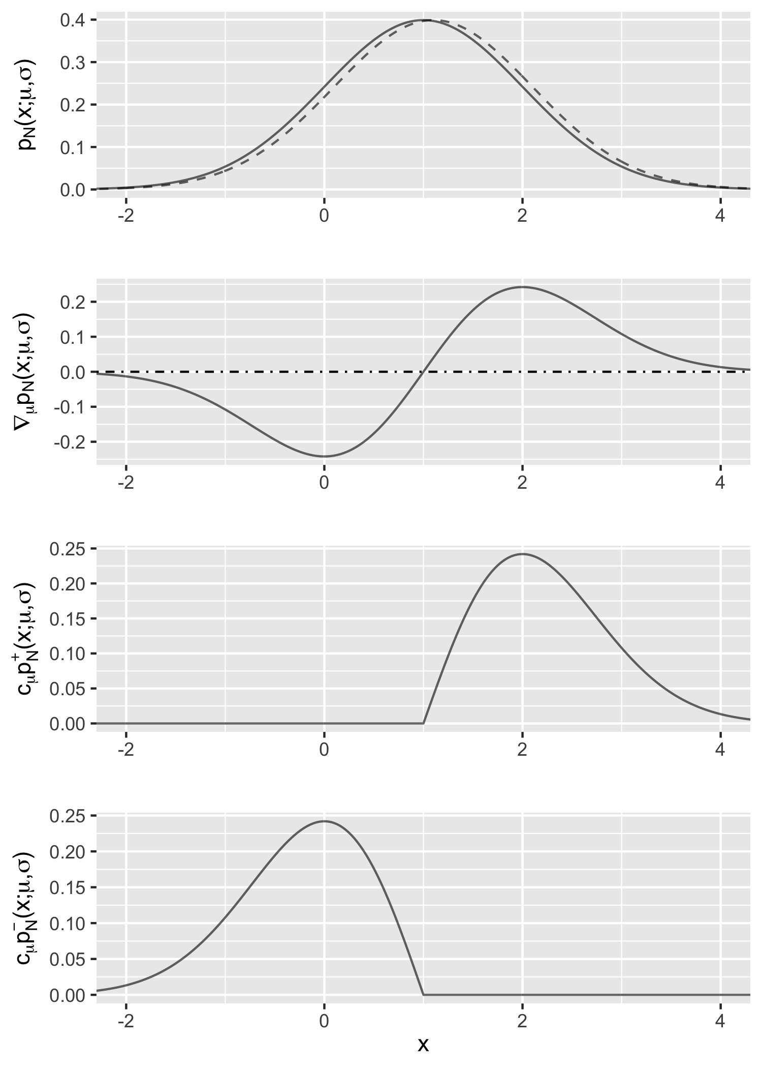
Example 1 (Normal distribution with respect to the location parameter). Consider the derivative of the density function of $\mathcal{N}(\mu, \sigma^2)$ with respect to $\mu$. We would like to show that \begin{equation} \nabla_\mu p_{\mathcal{N}}(x; \mu, \sigma) = c_\mu \left(p^+ (x; \mu, \sigma) - p^- (x; \mu, \sigma) \right), \label{eq:gaussian-mean} \tag{1} \end{equation} where

• $c_\mu = (\sigma \sqrt{2\pi})^{-1} $;
• $p^+$ is the density function of $\mu + \sigma \mathcal{W}(\lambda=\sqrt{2}, k=2)$;
• $p^-$ is the density function of $\mu - \sigma \mathcal{W}(\lambda=\sqrt{2}, k=2)$.

The notation $\mu \pm \sigma \mathcal{W}(\lambda=\sqrt{2}, k=2)$ represents a random variable $\mu \pm \sigma Y$, where $Y \sim \mathcal{W}(\lambda=\sqrt{2}, k=2)$, the Weibull distribution.

Proof. For the left-hand side of Equation \ref{eq:gaussian-mean}, basic calculus shows that $$ \nabla_{\mu} p_{\mathcal{N}}(x; \mu, \sigma) = \frac{x-\mu}{\sigma^3 \sqrt{2\pi}} \exp\left(- \frac{(x - \mu)^2}{2\sigma^2}\right). $$

Recall that the density function of a Weibull random variable $\mathcal{W}(\lambda=\sqrt{2}, k=2)$ is $$ p_\mathcal{W}(x; \lambda=\sqrt{2}, k=2) = x \exp\left( -\frac{x^2}{2} \right) \mathbb{I}_{x \geq 0}. $$ Using the change of variables formula, we have $$ p^+(x; \mu, \sigma) = \frac{x-\mu}{\sigma^2} \exp\left( -\frac{(x-\mu)^2}{2\sigma^2} \right) \mathbb{I}_{x \geq \mu} $$ and $$ p^-(x; \mu, \sigma) = -\frac{x-\mu}{\sigma^2} \exp\left( -\frac{(x-\mu)^2}{2\sigma^2} \right) \mathbb{I}_{x \leq \mu}. $$ Therefore, the right-hand side of Equation \ref{eq:gaussian-mean} is

$$ c_\mu \left(p^+ (x; \mu, \sigma) - p^- (x; \mu, \sigma) \right)= \frac{x-\mu}{\sigma^3 \sqrt{2\pi}} \exp\left(- \frac{(x - \mu)^2}{2\sigma^2}\right), $$ which equals the left-hand side.

Figure 1 gives an illustration of this example with $\mu=\sigma=1$. The first row shows the density function $p_{\mathcal{N}}(x; \mu, \sigma)$ (the solid line) and how it changes when $\mu$ increases by 0.1 (the dashed line); the difference (divided by 0.1) is approximately the gradient of interest. The second row is the gradient $\nabla_{\mu} p_{\mathcal{N}}(x; \mu, \sigma)$. The last two rows are the positive and negative components multiplied by the constant $c_\mu$, respectively; it indicates that the difference between them matches the curve in the second row.

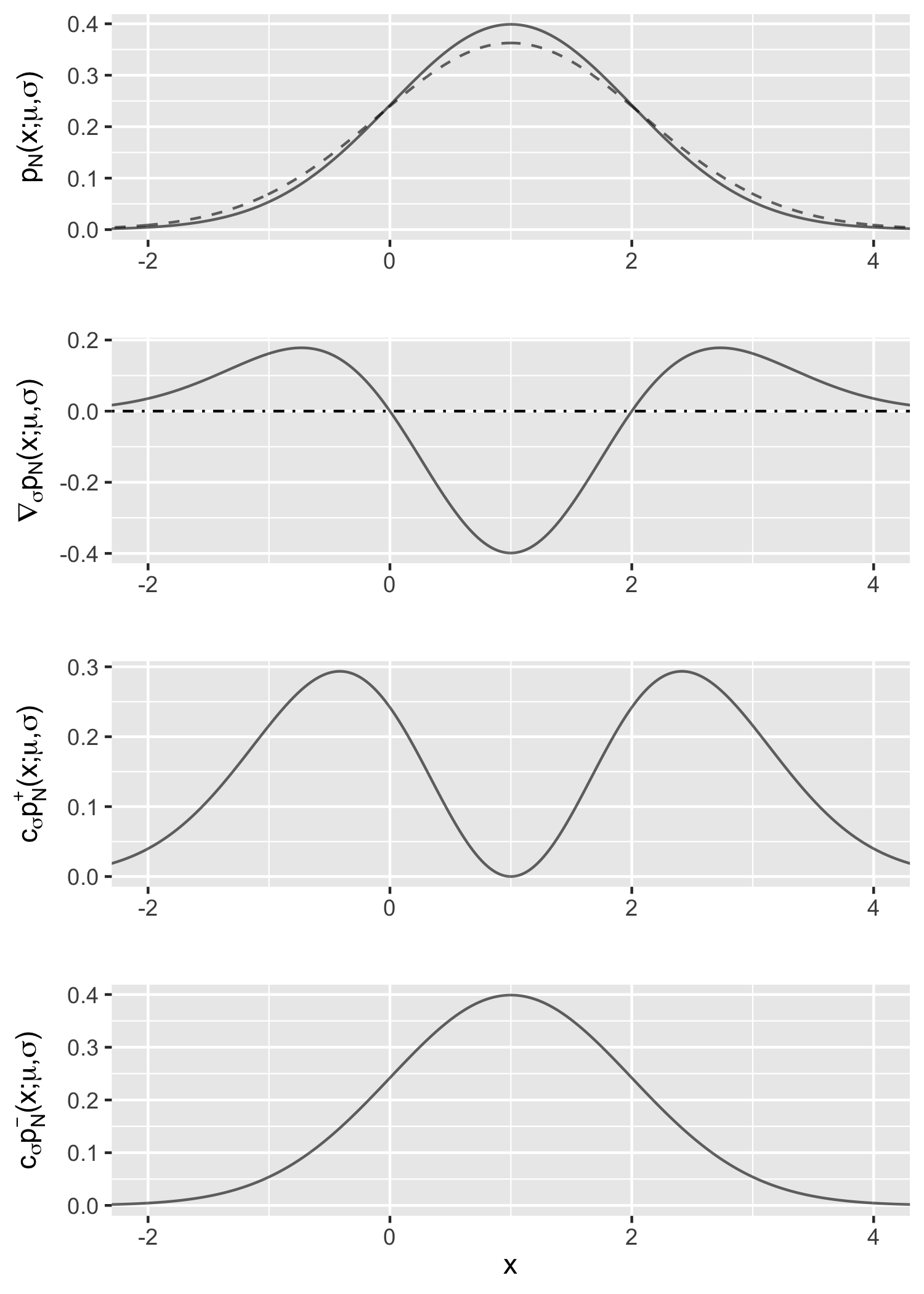
Example 2 (Normal distribution with respect to the scale parameter). Consider the derivative of the density function of $\mathcal{N}(\mu, \sigma^2)$ with respect to $\sigma$. We would like to show that \begin{equation} \nabla_\sigma p_{\mathcal{N}}(x; \mu, \sigma) = c_\sigma \left(p^+ (x; \mu, \sigma) - p^- (x; \mu, \sigma) \right), \label{eq:gaussian-std} \tag{2} \end{equation} where

• $c_\sigma = \sigma^{-1}$;
• $p^+ = p_\mathcal{M}(x; \mu, \sigma)$;
• $p^-= p_\mathcal{N}(x; \mu, \sigma)$.

Proof. The proof is similar to that of Example 1 using basic calculus: \begin{align} &\quad \nabla_{\sigma} p_{\mathcal{N}}(x; \mu, \sigma) \newline & = \frac{1}{\sigma} \left[ \frac{(x-\mu)^2}{\sigma^3 \sqrt{2\pi}} \exp\left(- \frac{(x - \mu)^2}{2\sigma^2}\right) - \frac{1}{\sigma \sqrt{2\pi}} \exp\left(- \frac{(x - \mu)^2}{2\sigma^2}\right) \right] \newline & = \sigma^{-1} \left( p_\mathcal{M}(x; \mu, \sigma) - p_\mathcal{N}(x; \mu, \sigma) \right). \end{align}

Figure 2 is the corresponding illustration.

2.3. Pros and cons

The advantage of the measure-valued gradient estimator is its flexibility. It is applicable to both continuous and discrete random variables. Also, unlike the pathwise estimator, it does not assume the function $f$ to be differentiable. Furthermore, there are distributions where the measure-valued gradient estimator is applicable, but the score function estimator is not, for example, the uniform distribution $\mathcal{U}(0, \theta)$.

One major disadvantage is its computational cost. The estimator only applies to a single parameter. For distributions with many parameters, it requires two forward passes of the function $f$ for each parameter, which might be computationally prohibitive.

3. Application to variational autoencoder

As mentioned before, the pathwise estimator or reparametrization trick is commonly used in variation inference, in particular, the variational autoencoder (VAE). The objective of VAE is to maximize the evidence lower bound (ELBO), $$ \mathcal{L} = \mathbb{E}_{\boldsymbol{z} \sim q_{\boldsymbol\phi}(\boldsymbol{z} | \boldsymbol{x})} \log ( p_{\boldsymbol\theta}(\boldsymbol{x} | \boldsymbol{z}) ) - D_{\mathrm{KL}} ( q_{\boldsymbol\phi}(\boldsymbol{z} | \boldsymbol{x}) \parallel p(\boldsymbol{z}) ), $$ where $D_{\mathrm{KL}}$ denotes the Kullback–Leibler divergence; $\boldsymbol{x}$ and $\boldsymbol{z}$ are the observed and latent variables, respectively; $p(\boldsymbol{z})$ is the prior distribution of $\boldsymbol{z}$; $p_{\boldsymbol\theta}(\boldsymbol{x} | \boldsymbol{z})$ is the generative distribution and is implemented by a decoding network parametrized by $\boldsymbol\theta$; $q_{\boldsymbol\phi}(\boldsymbol{z} | \boldsymbol{x})$ is the variational distribution and is implemented by an encoding network parametrized by $\boldsymbol\phi$.

Given a sample $\boldsymbol{z} \sim q_{\boldsymbol\phi}(\boldsymbol{z} | \boldsymbol{x})$, the gradient with respect to the decoder parameters $\nabla_{\boldsymbol\theta} \mathcal{L}$ can be easily obtained by automatic differentiation. Furthermore, if $p(\boldsymbol{z})$ and $q_{\boldsymbol\phi}(\boldsymbol{z} | \boldsymbol{x})$ are both diagonal Gaussians, the KL divergence has a closed-form expression, and $\nabla_{\boldsymbol\phi} D_{\mathrm{KL}} ( q_{\boldsymbol\phi}(\boldsymbol{z} | \boldsymbol{x}) \parallel p(\boldsymbol{z}) )$ can also be computed via automatic differentiation. However, to estimate $\nabla_{\boldsymbol\phi} \mathbb{E}_{\boldsymbol{z} \sim q_{\boldsymbol\phi}(\boldsymbol{z} | \boldsymbol{x})} \log ( p_{\boldsymbol\theta}(\boldsymbol{x} | \boldsymbol{z}) )$, a Monte Carlo gradient estimator is necessary. In this section, we demonstrate how to estimate it using the measure-valued gradient estimator. The code is adapted from the PyTorch VAE example.

We first define the VAE module. The encoder and decoder are both two-layer fully connected networks, with default arguments args.hidden_dim = 400 and args.z_dim = 20. The only difference from the original code is the line z = z.detach() in reparameterize(). This is to prevent the gradient $\nabla_{\boldsymbol\phi} \mathbb{E}_{\boldsymbol{z} \sim q_{\boldsymbol\phi}(\boldsymbol{z} | \boldsymbol{x})} \log ( p_{\boldsymbol\theta}(\boldsymbol{x} | \boldsymbol{z}) )$ from flowing into the encoder network.

Assuming $p_{\boldsymbol\theta}(\boldsymbol{x} | \boldsymbol{z})$ is a Bernoulli distribution, $\log p_{\boldsymbol\theta}(\boldsymbol{x} | \boldsymbol{z})$ is the binary cross entropy function and it is the integrand.

Next, we need to be able to sample from the Weibull distribution and double-sided Maxwell distribution. PyTorch has a built-in Weibull distribution class, and we can directly sample from an instance of that class. For the double-sided Maxwell distribution, we can use the following property to sample from $\mathcal{M}(0, 1)$:

If $X \sim \mathrm{Bernoulli}(1/2)$, $Y \sim \mathrm{Gamma}(3/2, 1/2)$, and $X$ and $Y$ are independent, then $(2X - 1) \sqrt{Y} \sim \mathcal{M}(0, 1)$.

Now we are ready to introduce the most crucial function get_mu_std_grad(). It returns the estimated gradient of $\mathbb{E}_{\boldsymbol{z} \sim q_{\boldsymbol\phi}(\boldsymbol{z} | \boldsymbol{x})} \log ( p_{\boldsymbol\theta}(\boldsymbol{x} | \boldsymbol{z}) )$ with respect to mu and std, the output of encode() in the VAE class.

The idea is to draw two samples z1 and z2 from the variational distribution first. Then, we loop through all the latent dimensions; in the $i$-th iteration, z1 and z2 are cloned to z1_copy and z2_copy, then the $i$-th elements of z1_copy and z2_copy are substituted with samples from $p^+$ and $p^-$, respectively. Finally, the updated z1_copy and z2_copy are passed to the function f_integrand, and the difference divided by the constant is the resulting gradient estimate for the $i$-th parameter.

It is worth mentioning that when estimating the gradient with respect to the standard deviation $\sigma$, the two samples from $\mathcal{M}(x; \mu, \sigma)$ and $\mathcal{N}(x; \mu, \sigma)$ are not independent. We first draw a sample from the positive component $\hat{x}^+ \sim \mathcal{M}(x; \mu, \sigma)$, then draw a uniform sample $\hat{u} \sim \mathcal{U}(0, 1)$, finally set $\hat{x}^- := \hat{u} \cdot \hat{x}^+$. It can be shown that $\hat{x}^- \sim \mathcal{N}(x; \mu, \sigma)$, the negative component. This is a variance reduction method known as the Maxwell-Gaussian coupling.

Finally, everything is put together to the train() function. The gradients of the decoder come from the binary cross-entropy loss; the gradients of the encoder come from two sources: the KL divergence and the measure-valued gradient estimator.

Complete code can be found in the next section.

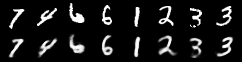
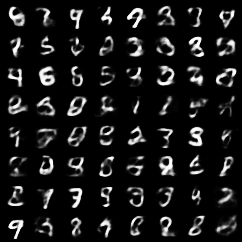
Figures 3 and 4 show the reconstructed images and the generated images with a model trained for 10 epochs. Qualitatively, the results seem reasonable.

4. Complete code

References

• Mohamed, S., Rosca, M., Figurnov, M., & Mnih, A. (2019). Monte Carlo gradient estimation in machine learning. arXiv preprint arXiv:1906.10652.