Understanding Shapes in PyTorch Distributions Package
The torch.distributions package implements various probability distributions, as well as methods for sampling and computing statistics.
It generally follows the design of the TensorFlow distributions package (Dillon et al. 2017).
There are three types of “shapes”, sample shape, batch shape, and event shape, that are crucial to understanding the torch.distributions package.
The same definition of shapes is also used in other packages, including GluonTS, Pyro, etc.
In this blog post, we describe the different types of shapes and illustrate the differences among them by code examples.
On top of that, we try to answer a few questions related to the shapes in torch.distributions.
All code examples are compatible with PyTorch v1.3.0.
Three types of shapes
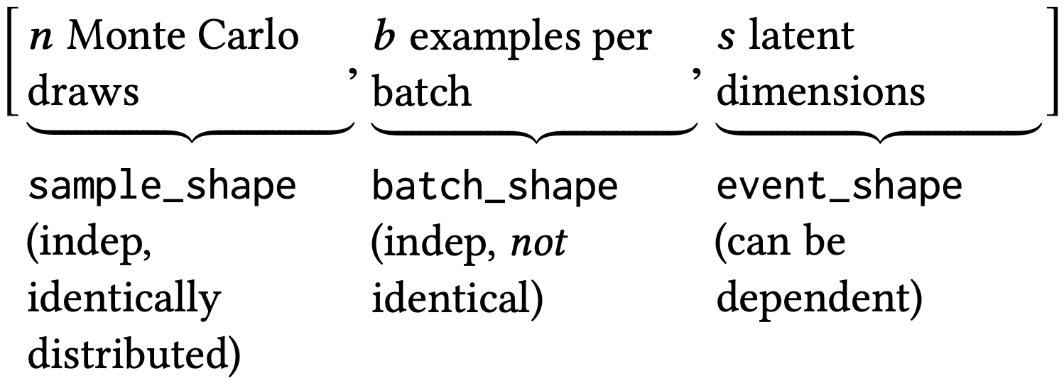
The three types of shapes are defined as follows and illustrated in Figure 1.
- Sample shape describes independent, identically distributed draws from the distribution.
- Batch shape describes independent, not identically distributed draws. Namely, we may have a set of (different) parameterizations to the same distribution. This enables the common use case in machine learning of a batch of examples, each modeled by its own distribution.
- Event shape describes the shape of a single draw (event space) from the distribution; it may be dependent across dimensions.
The definitions above might be difficult to understand.
We take the Monte Carlo estimation of the evidence lower bound (ELBO) in the variational autoencoder (VAE) as an example to illustrate their differences.
The average ELBO over a batch of $b$ observations, $x_i$ for $i=1,\ldots,b$, is
$$
\mathcal{L} =
\frac{1}{b}
\sum_{i=1}^b
\mathbb{E}_{q(z|x_i)}
\log\left[ \frac{p(x_i | z) p(z)}{q(z | x_i)} \right],
$$
where $z \in \mathbb{R}^s$ is an $s$-dimensional latent vector.
The ELBO can be estimated by Monte Carlo samples; specifically, for each $x_i$, $n$ samples are drawn from $z_{ij} \overset{\text{i.i.d.}}{\sim} q(z|x_i)$ for $j = 1, \ldots, n$.
The estimate is then
$$
\widehat{\mathcal{L}} =
\frac{1}{bn}
\sum_{i=1}^b
\sum_{j=1}^n
\log\left[ \frac{p(x_i | z_{ij}) p(z_{ij})}{q(z_{ij} | x_i)} \right].
$$
All the Monte Carlos samples $z_{ij}$ can be compactly represented as a tensor of shape $(n, b, s)$ or, correspondingly, [sample_shape, batch_shape, event_shape].
We also provide mathematical notations for a few combinations of shapes in Table 1, for Gaussian random variables/vectors.
Ignoring subscripts, $X$ represents a random variable, $\mu$ and $\sigma$ are scalars;
$\mathbf{X}$ denotes a two-dimensional random vector, $\boldsymbol\mu$ is a two-dimensional vector, and $\boldsymbol\Sigma$ is a $2 \times 2$ (not necessarily diagonal) matrix.
Moreover, [] and [2] denote torch.Size([]) and torch.Size([2]), respectively.
For each row, the link to a PyTorch code example is also given.
| no. | sample shape | batch shape | event shape | mathematical notation | code |
|---|---|---|---|---|---|
| 1 | [] |
[] |
[] |
$X \sim \mathcal{N}(\mu, \sigma^2)$ | link |
| 2 | [2] |
[] |
[] |
$X_1, X_2 \overset{\text{i.i.d.}}{\sim} \mathcal{N}(\mu, \sigma^2)$ | link |
| 3 | [] |
[2] |
[] |
$X_1 \sim \mathcal{N}(\mu_1, \sigma_1^2)$ $X_2 \sim \mathcal{N}(\mu_2, \sigma_2^2)$ |
link |
| 4 | [] |
[] |
[2] |
$\mathbf{X} \sim \mathcal{N}(\boldsymbol\mu, \boldsymbol\Sigma)$ | link |
| 5 | [] |
[2] |
[2] |
$\mathbf{X}_1 \sim \mathcal{N}(\boldsymbol\mu_1, \boldsymbol\Sigma_1)$ $\mathbf{X}_2 \sim \mathcal{N}(\boldsymbol\mu_2, \boldsymbol\Sigma_2)$ |
link |
| 6 | [2] |
[] |
[2] |
$\mathbf{X}_1, \mathbf{X}_2 \overset{\text{i.i.d.}}{\sim} \mathcal{N}(\boldsymbol\mu, \boldsymbol\Sigma)$ | link |
| 7 | [2] |
[2] |
[] |
$X_{11}, X_{12} \overset{\text{i.i.d.}}{\sim} \mathcal{N}(\mu_1, \sigma_1^2)$ $X_{21}, X_{22} \overset{\text{i.i.d.}}{\sim} \mathcal{N}(\mu_2, \sigma_2^2)$ |
link |
| 8 | [2] |
[2] |
[2] |
$\mathbf{X}_{11}, \mathbf{X}_{12} \overset{\text{i.i.d.}}{\sim} \mathcal{N}(\boldsymbol\mu_1, \boldsymbol\Sigma_1)$ $\mathbf{X}_{21}, \mathbf{X}_{22} \overset{\text{i.i.d.}}{\sim} \mathcal{N}(\boldsymbol\mu_2, \boldsymbol\Sigma_2)$ |
link |
This table is adapted from this blog post; you might find the visualization in that post helpful.
Every Distribution class has instance attributes batch_shape and event_shape.
Furthermore, each class also has a method .sample, which takes sample_shape as an argument and generates samples from the distribution.
Note that sample_shape is not an instance attribute because, conceptually, it is not associated with a distribution.
What is the difference between Normal and MultivariateNormal?
There are two distribution classes that correspond to normal distributions: the univariate normal
torch.distributions.normal.Normal(loc, scale, validate_args=None)
and the multivariate normal
torch.distributions.multivariate_normal.MultivariateNormal(loc,
covariance_matrix=None, precision_matrix=None, scale_tril=None,
validate_args=None)
Since the Normal class represents univariate normal distributions, the event_shape of a Normal instance is always torch.Size([]).
Even if the loc or scale arguments are high-order tensors, their “shapes” will go to batch_shape.
For example,
>>> normal = Normal(torch.randn(5, 3, 2), torch.ones(5, 3, 2))
>>> (normal.batch_shape, normal.event_shape)
(torch.Size([5, 3, 2]), torch.Size([]))
In contrast, for MultivariateNormal, the batch_shape and event_shape can be inferred from the shape of covariance_matrix.
In the following example, the covariance matrix torch.eye(2) is $2 \times 2$ matrix, so it can be inferred that the event_shape should be [2] and the batch_shape is [5, 3].
>>> mvn = MultivariateNormal(torch.randn(5, 3, 2), torch.eye(2))
>>> (mvn.batch_shape, mvn.event_shape)
(torch.Size([5, 3]), torch.Size([2]))
What does .expand do?
Every Distribution instance has an .expand method. Its docstring is as follows:
class Distribution(object):

    def expand(self, batch_shape, _instance=None):
        """
        Returns a new distribution instance (or populates an existing instance
        provided by a derived class) with batch dimensions expanded to
        `batch_shape`. This method calls :class:`~torch.Tensor.expand` on
        the distribution's parameters. As such, this does not allocate new
        memory for the expanded distribution instance. Additionally,
        this does not repeat any args checking or parameter broadcasting in
        `__init__.py`, when an instance is first created.

        Args:
            batch_shape (torch.Size): the desired expanded size.
            _instance: new instance provided by subclasses that
                need to override `.expand`.

        Returns:
            New distribution instance with batch dimensions expanded to
            `batch_size`.
        """
        raise NotImplementedError
It essentially creates a new distribution instance by expanding the batch_shape.
For example, if we define a MultivariateNormal instance with a batch_shape of [] and an event_shape of [2],
>>> mvn = MultivariateNormal(torch.randn(2), torch.eye(2))
>>> (mvn.batch_shape, mvn.event_shape)
(torch.Size([]), torch.Size([2]))
it can be expanded to a new instance that have a batch_shape of [5]:
>>> new_batch_shape = torch.Size([5])
>>> expanded_mvn = mvn.expand(new_batch_shape)
>>> (expanded_mvn.batch_shape, expanded_mvn.event_shape)
(torch.Size([5]), torch.Size([2]))
Note that no new memory is allocated in this process; therefore, all batch dimensions have the same location parameter.
>>> expanded_mvn.loc
tensor([[-2.2299,  0.0122],
        [-2.2299,  0.0122],
        [-2.2299,  0.0122],
        [-2.2299,  0.0122],
        [-2.2299,  0.0122]])
This can be compared with the following example with the same batch_shape of [5] and event_shape of [2].
However, the batch dimensions have different location parameters.
>>> batched_mvn = MultivariateNormal(torch.randn(5, 2), torch.eye(2))
>>> (batched_mvn.batch_shape, batched_mvn.event_shape)
(torch.Size([5]), torch.Size([2]))
>>> batched_mvn.loc
tensor([[-0.3935, -0.7844],
        [ 0.3310,  0.9311],
        [-0.8141, -0.2252],
        [ 2.4199, -0.5444],
        [ 0.5586,  1.0157]])
What is the Independent class?
The Independent class does not represent any probability distribution.
Instead, it creates a new distribution instance by “reinterpreting” some of the batch shapes of an existing distribution as event shapes.
torch.distributions.independent.Independent(base_distribution,
reinterpreted_batch_ndims, validate_args=None)
The first argument base_distribution is self-explanatory; the second argument reinterpreted_batch_ndims is the number of batch shapes to be reinterpreted as event shapes.
The usage of the Independent class can be illustrated by the following example.
We start with a Normal instance with a batch_shape of [5, 3, 2] and an event_shape of [].
>>> loc = torch.zeros(5, 3, 2)
>>> scale = torch.ones(2)
>>> normal = Normal(loc, scale)
>>> [normal.batch_shape, normal.event_shape]
[torch.Size([5, 3, 2]), torch.Size([])]
An Independent instance can reinterpret the last batch_shape as the event_shape.
As a result, the new batch_shape is [5, 3], and the event_shape now becomes [2].
>>> normal_ind_1 = Independent(normal, 1)
>>> [normal_ind_1.batch_shape, normal_ind_1.event_shape]
[torch.Size([5, 3]), torch.Size([2])]
The instance normal_ind_1 is essentially the same as the following MultivariateNormal instance:
>>> mvn = MultivariateNormal(loc, torch.diag(scale))
>>> [mvn.batch_shape, mvn.event_shape]
[torch.Size([5, 3]), torch.Size([2])]
We can further reinterpret more batch shapes as event shapes:
>>> normal_ind_1_ind_1 = Independent(normal_ind_1, 1)
>>> [normal_ind_1_ind_1.batch_shape, normal_ind_1_ind_1.event_shape]
[torch.Size([5]), torch.Size([3, 2])
or equivalently,
>>> normal_ind_2 = Independent(normal, 2)
>>> [normal_ind_2.batch_shape, normal_ind_2.event_shape]
[torch.Size([5]), torch.Size([3, 2])]
PyTorch code examples
In this section, code examples for each row in the Table 1 are provided.
The following import statements are needed for the examples.
import torch
from torch.distributions.normal import Normal
from torch.distributions.multivariate_normal import MultivariateNormal
Row 1: [], [], []
>>> dist = Normal(0.0, 1.0)
>>> sample_shape = torch.Size([])
>>> dist.sample(sample_shape)
tensor(-1.3349)
>>> (sample_shape, dist.batch_shape, dist.event_shape)
(torch.Size([]), torch.Size([]), torch.Size([]))
Row 2: [2], [], []
>>> dist = Normal(0.0, 1.0)
>>> sample_shape = torch.Size([2])
>>> dist.sample(sample_shape)
tensor([ 0.2786, -1.4113])
>>> (sample_shape, dist.batch_shape, dist.event_shape)
(torch.Size([2]), torch.Size([]), torch.Size([]))
Row 3: [], [2], []
>>> dist = Normal(torch.zeros(2), torch.ones(2))
>>> sample_shape = torch.Size([])
>>> dist.sample(sample_shape)
tensor([0.0101, 0.6976])
>>> (sample_shape, dist.batch_shape, dist.event_shape)
(torch.Size([]), torch.Size([2]), torch.Size([]))
Row 4: [], [], [2]
>>> dist = MultivariateNormal(torch.zeros(2), torch.eye(2))
>>> sample_shape = torch.Size([])
>>> dist.sample(sample_shape)
tensor([ 0.2880, -1.6795])
>>> (sample_shape, dist.batch_shape, dist.event_shape)
(torch.Size([]), torch.Size([]), torch.Size([2]))
Row 5: [], [2], [2]
>>> dist = MultivariateNormal(torch.zeros(2, 2), torch.eye(2))
>>> sample_shape = torch.Size([])
>>> dist.sample(sample_shape)
tensor([[-0.4703,  0.4152],
        [-1.6471, -0.6276]])
>>> (sample_shape, dist.batch_shape, dist.event_shape)
(torch.Size([]), torch.Size([2]), torch.Size([2]))
Row 6: [2], [], [2]
>>> dist = MultivariateNormal(torch.zeros(2), torch.eye(2))
>>> sample_shape = torch.Size([2])
>>> dist.sample(sample_shape)
tensor([[ 2.2040, -0.7195],
        [-0.4787,  0.0895]])
>>> (sample_shape, dist.batch_shape, dist.event_shape)
(torch.Size([2]), torch.Size([]), torch.Size([2]))
Row 7: [2], [2], []
>>> dist = Normal(torch.zeros(2), torch.ones(2))
>>> sample_shape = torch.Size([2])
>>> dist.sample(sample_shape)
tensor([[ 0.2639,  0.9083],
        [-0.7536,  0.5296]])
>>> (sample_shape, dist.batch_shape, dist.event_shape)
(torch.Size([2]), torch.Size([2]), torch.Size([]))
Row 8: [2], [2], [2]
>>> dist = MultivariateNormal(torch.zeros(2, 2), torch.eye(2))
>>> sample_shape = torch.Size([2])
>>> dist.sample(sample_shape)
tensor([[[ 0.4683,  0.6118],
         [ 1.0697, -0.0856]],

        [[-1.3001, -0.1734],
         [ 0.4705, -0.0404]]])
>>> (sample_shape, dist.batch_shape, dist.event_shape)
(torch.Size([2]), torch.Size([2]), torch.Size([2]))
References
- Dillon, J. V., Langmore, I., Tran, D., Brevdo, E., Vasudevan, S., Moore, D., … & Saurous, R. A. (2017). Tensorflow distributions. arXiv preprint arXiv:1711.10604.