Traveling Salesman Problem and Approximation Algorithms

One of my research interests is a graphical model structure learning problem in multivariate statistics. I have been recently studying and trying to borrow ideas from approximation algorithms, a research field that tackles difficult combinatorial optimization problems. This post gives a brief introduction to two approximation algorithms for the (metric) traveling salesman problem: the double-tree algorithm and Christofides’ algorithm. The materials are mainly based on §2.4 of Williamson and Shmoys (2011).

1. Approximation algorithms

In combinatorial optimization, most interesting problems are NP-hard and do not have polynomial-time algorithms to find optimal solutions (yet?). Approximation algorithms are efficient algorithms that find approximate solutions to such problems. Moreover, they give provable guarantees on the distance of the approximate solution to the optimal ones.

We assume that there is an objective function associated with an optimization problem. An optimal solution to the problem is one that minimizes the value of this objective function. The value of the optimal solution is often denoted by $\mathrm{OPT}$.

An $\alpha$-approximation algorithm for an optimization problem is a polynomial-time algorithm that for all instances of the problem produces a solution, whose value is within a factor of $\alpha$ of $\mathrm{OPT}$, the value of an optimal solution. The factor $\alpha$ is called the approximation ratio.

2. Traveling salesman problem

The traveling salesman problem (TSP) is NP-hard and one of the most well-studied combinatorial optimization problems. It has broad applications in logistics, planning, and DNA sequencing. In plain words, the TSP asks the following question:

Given a list of cities and the distances between each pair of cities, what is the shortest possible route that visits each city and returns to the origin city?

Formally, for a set of cities $[n] = \{1, 2, \ldots, n \}$, an $n$-by-$n$ matrix $C = (c_{ij})$, where $c_{ij} \geq 0 $ specifies the cost of traveling from city $i$ to city $j$. By convention, we assume $c_{ii} = 0$ and $c_{ij} = c_{ji}$, meaning that the cost of traveling from city $i$ to city $j$ is equal to the cost of traveling from city $j$ to city $i$. Furthermore, we only consider the metric TSP in this article; that is, the triangle inequality holds for any $i,j,k$: $$ c_{ik} \leq c_{ij} + c_{jk}, \quad \forall i, j, k \in [n]. $$

Given a permutation $\sigma$ of $[n]$, a tour traverses the cities in the order $\sigma(1), \sigma(2), \ldots, \sigma(n)$. The goal is to find a tour with the lowest cost, which is equal to $$ c_{\sigma(n) \sigma(1)} + \sum_{i=1}^{n-1} c_{\sigma(i) \sigma(i+1)}. $$

3. Double-tree algorithm

We first describe a simple algorithm called the double-tree algorithm and prove that it is a 2-approximation algorithm.

Double-tree algorithm

Find a minimum spanning tree $T$.

Duplicate the edges of $T$. Find an Eulerian tour.

Shortcut the Eulerian tour.

Figure 1 shows the algorithm on a simple five-city instance. We give a step-by-step explanation of the algorithm.

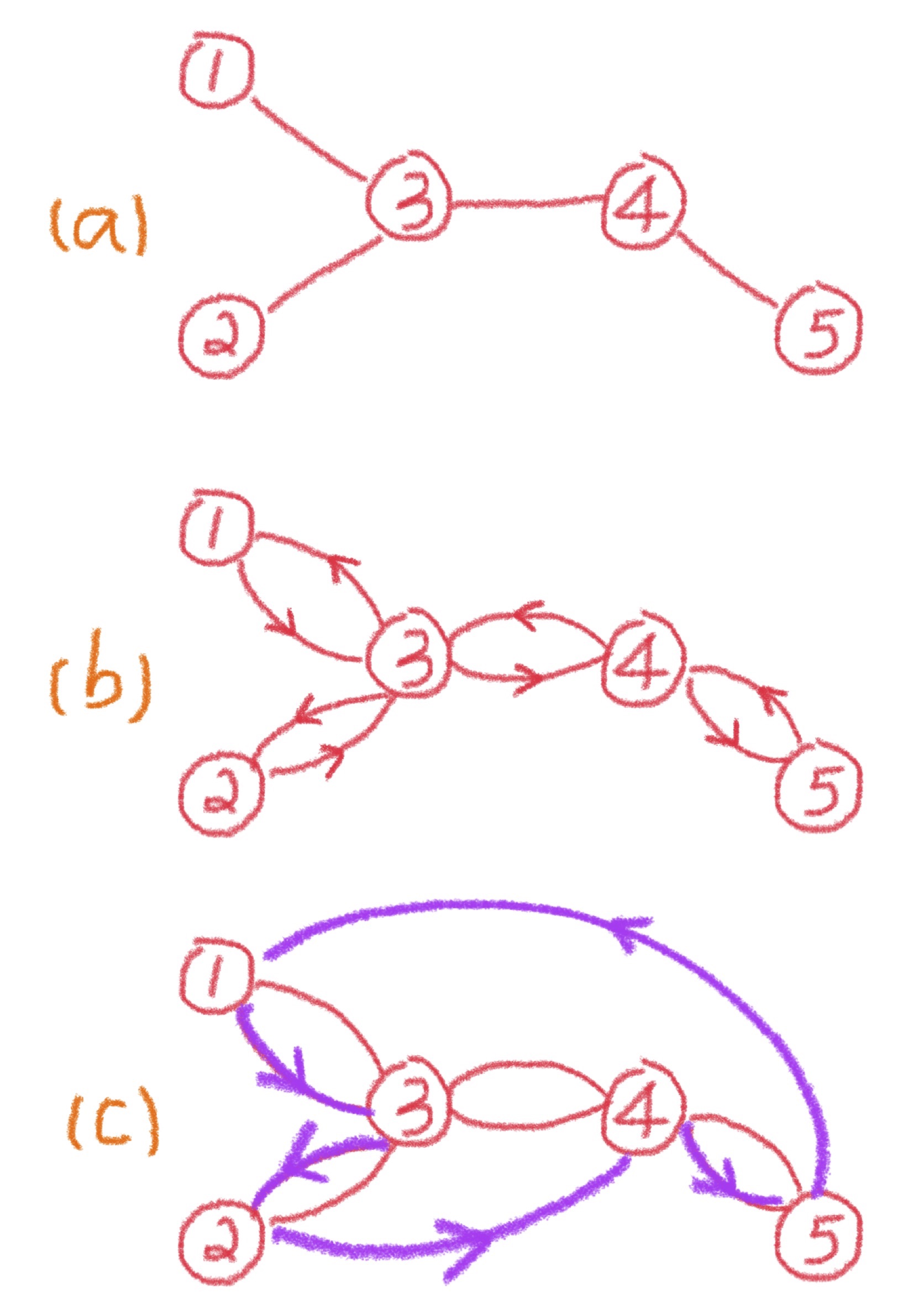
A spanning tree of an undirected graph is a subgraph that is a tree and includes all of the nodes. A minimum spanning tree of a weighted graph is a spanning tree for which the total edge cost is minimized. There are several polynomial-time algorithms for finding a minimum spanning tree, e.g., Prim’s algorithm, Kruskal’s algorithm, and the reverse-delete algorithm. Figure 1a shows a minimum spanning tree $T$.

There is an important relationship between the minimum spanning tree problem and the traveling salesman problem.

Lemma 1. For any input to the traveling salesman problem, the cost of the optimal tour is at least the cost of the minimum spanning tree on the same input.

The proof is simple. Deleting any edge from the optimal tour results in a spanning tree, the cost of which is at least the cost of the minimum spanning tree. Therefore, the cost of the minimum spanning tree $T$ in Figure 1(a) is at most $ \mathrm{OPT}$.

Next, each edge in the minimum spanning tree is replaced by two copies of itself, as shown in Figure 1b. The resulting (multi)graph is Eulerian. A graph is said to be Eulerian if there exists a tour that visits every edge exactly once. A graph is Eulerian if and only if it is connected and each node has an even degree. Given an Eulerian graph, it is easy to construct a traversal of the edges. For example, a possible Eulerian tour in Figure 1b is 1–3–2–3–4–5–4–3–1. Moreover, since the edges are duplicated from the minimum spanning tree, the Eulerian tour has cost at most $2 , \mathrm{OPT}$.

Finally, given the Eulerian tour, we remove all but the first occurrence of each node in the sequence; this step is called shortcutting. By the triangle inequality, the cost of the shortcut tour is at most the cost of the Eulerian tour, which is not greater than $2 , \mathrm{OPT}$. In Figure 1c, the shortcut tour is 1–3–2–4–5–1. When going from node 2 to node 4 by omitting node 3, we have $c_{24} \leq c_{23} + c_{34}$. Similarly, when skipping nodes 4 and 3, $c_{51} \leq c_{54} + c_{43} + c_{31}$.

Therefore, we have analyzed the approximation ratio of the double-tree algorithm.

Theorem 1. The double-tree algorithm for the metric traveling salesman problem is a 2-approximation algorithm.

4. Christofides' algorithm

The basic strategy of the double-tree algorithm is to construct an Eulerian tour whose total cost is at most $\alpha , \mathrm{OPT}$, then shortcut it to get an $\alpha$-approximation solution. The same strategy can be carried out to yield a 3/2-approximation algorithm.

Christofides' algorithm

Find a minimum spanning tree $T$.

Let $O$ be the set of nodes with odd degree in $T$. Find a minimum-cost perfect matching $M$ on $O$.

Add the set of edges of $M$ to $T$. Find an Eulerian tour.

Shortcut the Eulerian tour.

Figure 2 illustrates the algorithm on a simple five-city instance of TSP.

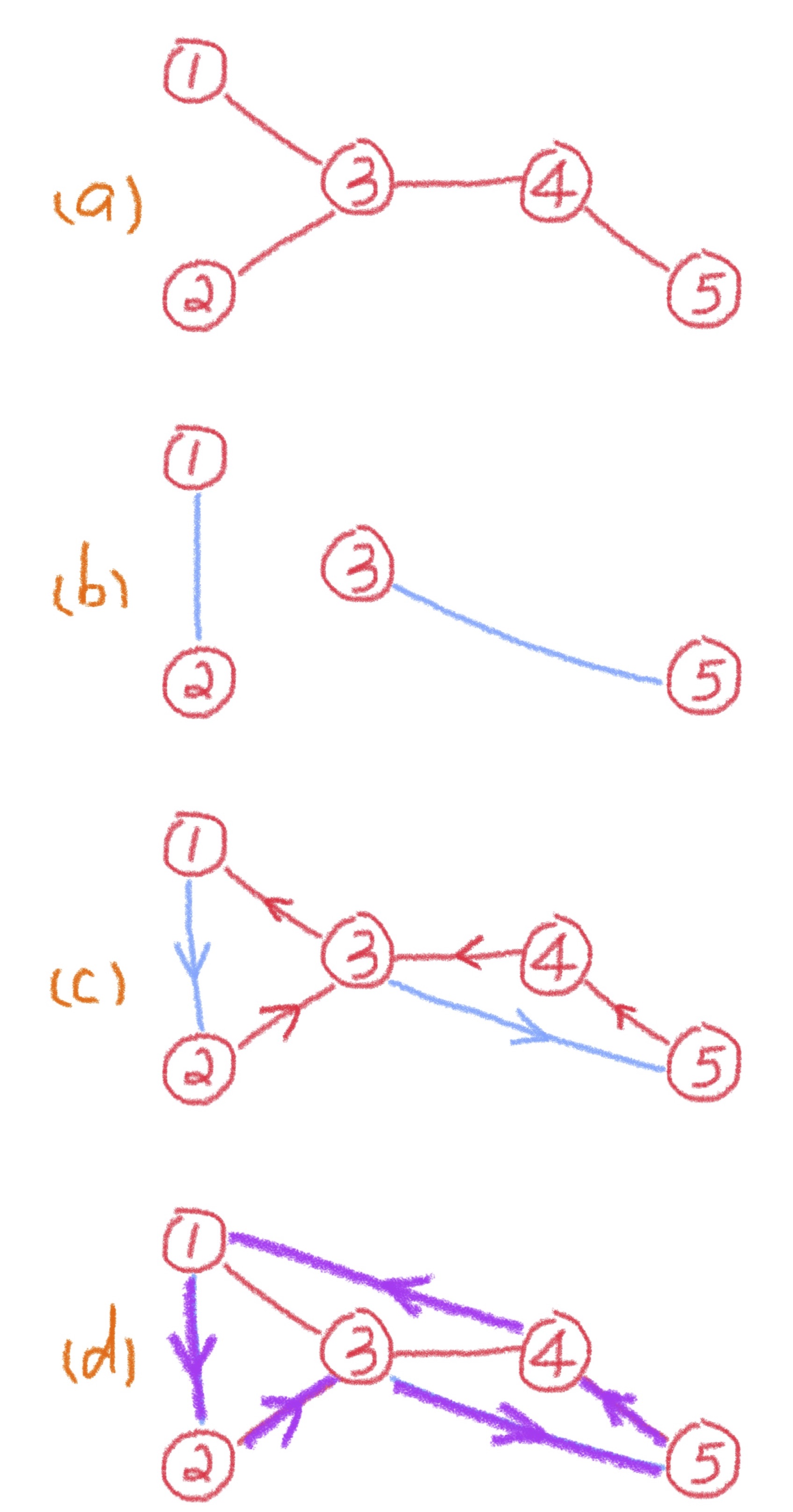
The algorithm starts again with the minimum spanning tree $T$. The reason we cannot directly find an Eulerian tour is that its leaf nodes all have degrees of one. However, by the handshaking lemma, there is an even number of odd-degree nodes. If these nodes can be paired up, then it becomes an Eulerian graph and we can proceed as before.

Let $O$ be the set of odd-degree nodes in $T$. To pair them up, we want to find a collection of edges that contain each node in $O$ exactly once. This is called a perfect matching in graph theory. Given a complete graph (on an even number of nodes) with edge costs, there is a polynomial-time algorithm to find the perfect matching of the minimum total cost, known as the blossom algorithm.

For the minimum spanning tree $T$ in Figure 2a, $ O = \{1, 2, 3, 5\}$. The minimum-cost perfect matching $M$ on the complete graph induced by $O$ is shown in Figure 2b. Adding the edges of $M$ to $T$, the result is an Eulerian graph, since we have added a new edge incident to each odd-degree node in $T$. The remaining steps are the same as in the double-tree algorithm.

We want to show that the Eulerian graph has total cost of at most 3/2 $\mathrm{OPT}$. Since the total cost of the minimum spanning tree $T$ is at most $\mathrm{OPT}$, we only need to show that the perfect matching $M$ has cost at most 1/2 $\mathrm{OPT}$.

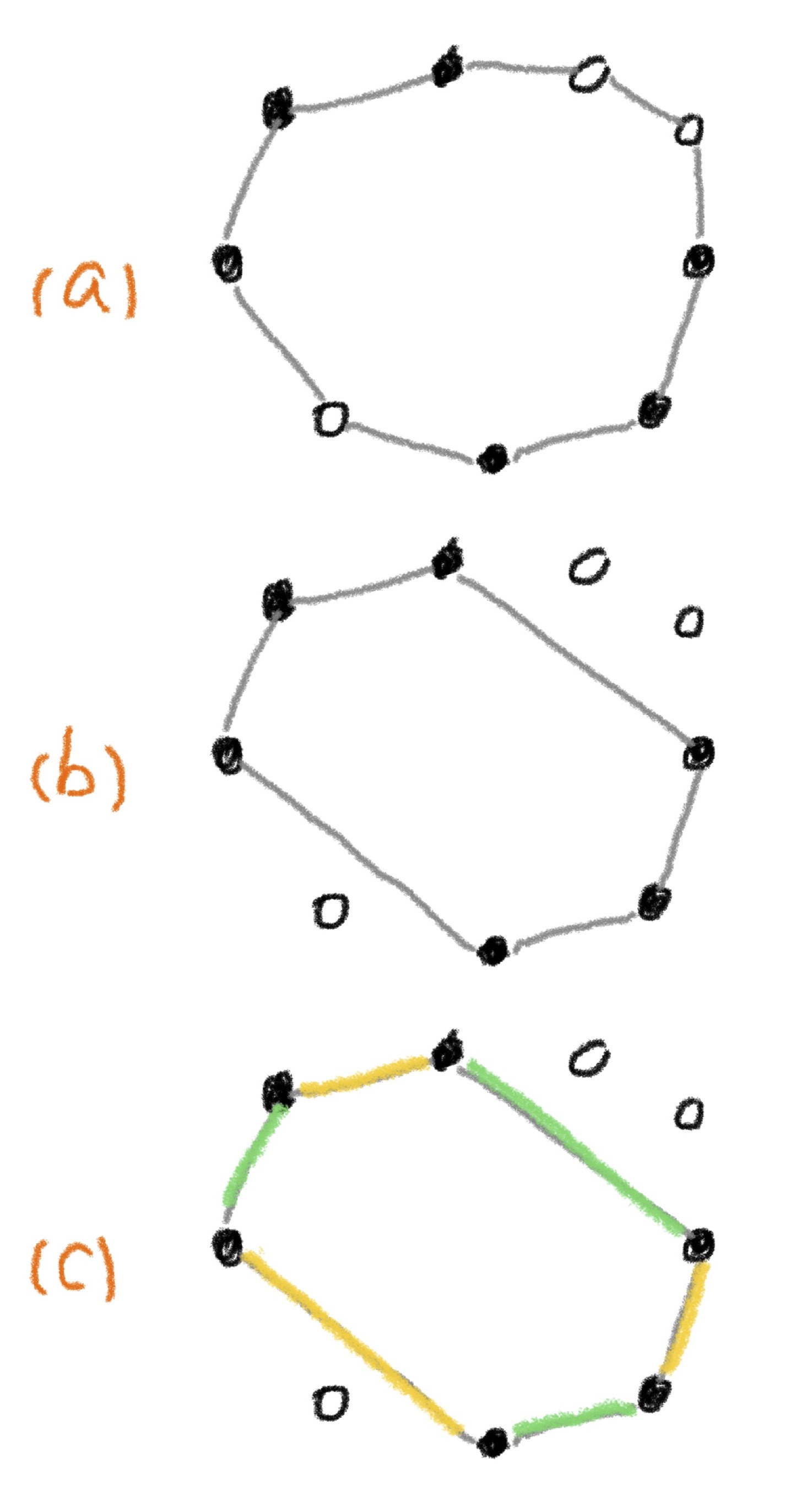
We start with the optimal tour on the entire set of cities, the cost of which is $\mathrm{OPT}$ by definition. Figure 3a presents a simplified illustration of the optimal tour; the solid circles represent nodes in $O$. By omitting the nodes that are not in $O$ from the optimal tour, we get a tour on $O$, as shown in Figure 3b. By the shortcutting argument again, the total cost of the tour on $O$ is at most $\mathrm{OPT}$. Next, color the edges yellow and green, alternating colors as the tour is traversed, as illustrated in Figure 3c. This partitions the edges into two sets: the yellow set and the green set; each is a perfect matching on $O$. Since the total cost of the two matchings is at most $\mathrm{OPT}$, the cheaper one has cost at most 1/2 $\mathrm{OPT}$. In other words, there exists a perfect matching on $O$ of cost at most 1/2 $\mathrm{OPT}$. Therefore, the minimum-cost perfect matching must have cost not greater than 1/2 $\mathrm{OPT}$. This completes the proof of the following theorem.

Theorem 2. Christofides' algorithm for the metric traveling salesman problem is a 3/2-approximation algorithm.

minimum-cost perfect matching — Figure 3: Minimum-cost perfect matching.

References

Williamson, D. P., & Shmoys, D. B. (2011). The Design of Approximation Algorithms. Cambridge University Press.